Advanced Risk Management Framework for FX and Commodity Trading

In today’s interconnected global markets, traditional correlation assumptions between gold and USD pairs can break down without warning, exposing portfolios to unexpected risks. This comprehensive guide provides institutional-grade methodologies for building robust risk management systems that adapt to changing market conditions. Drawing from over two decades of quantitative research and real-world trading experience, we present actionable frameworks that have been tested across multiple market cycles.

Part 1: Handling Correlation Breakdown Between Gold and USD Pairs

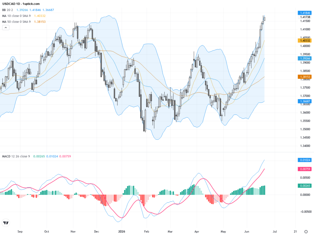
step_num: 1, heading: Understand the Traditional Gold-USD Relationship, content: Historically, gold and USD exhibit a negative correlation averaging -0.40 to -0.60 over long periods. This inverse relationship stems from gold being priced in dollars, safe-haven dynamics, and inflation hedging properties. However, this correlation can shift dramatically during regime changes, liquidity crises, or monetary policy pivots. Document your baseline correlation assumptions using rolling 60-day, 120-day, and 252-day windows to establish reference points.

step_num: 2, heading: Implement Real-Time Correlation Monitoring Systems, content: Deploy automated monitoring that tracks correlation coefficients across multiple timeframes. Set alert thresholds when correlations deviate by more than 1.5 standard deviations from historical norms. Use tools like DCC-GARCH (Dynamic Conditional Correlation) models to capture time-varying correlations. Create dashboards displaying correlation heatmaps updated at minimum daily frequency.

step_num: 3, heading: Identify Correlation Breakdown Catalysts, content: Build a checklist of events that historically trigger correlation breakdowns: Federal Reserve policy shifts, geopolitical crises, liquidity crunches, and risk-off episodes. During the 2008 financial crisis and March 2020 COVID crash, gold and USD temporarily moved together as both served as safe havens. Monitor these catalysts through news feeds and economic calendars integrated into your trading systems.

step_num: 4, heading: Develop Contingency Trading Protocols, content: Create pre-defined response protocols for correlation breakdown scenarios. Options include: reducing position sizes by 30-50% when correlations breach thresholds, implementing temporary hedges using options, or switching to regime-specific models. Document these protocols in your risk management playbook and conduct quarterly drills to ensure execution readiness.

step_num: 5, heading: Recalibrate Models Post-Breakdown, content: After correlation normalizes, conduct post-mortem analysis to understand what drove the breakdown and how your systems performed. Update your correlation models with recent data, potentially using exponentially weighted moving averages that give more weight to recent observations. Refine your early warning indicators based on lessons learned.

Part 2: Integrating Macro Regimes into FX and Commodity Risk Management

step_num: 1, heading: Define Your Macro Regime Classification System, content: Establish clear definitions for macro regimes relevant to FX and commodities: Growth/Inflation combinations (Goldilocks, Reflation, Stagflation, Deflation), Risk-On/Risk-Off states, and Monetary Policy regimes (Hawkish, Neutral, Dovish). Use quantitative indicators such as PMI trends, inflation breakevens, and central bank policy rates to classify current regimes objectively.

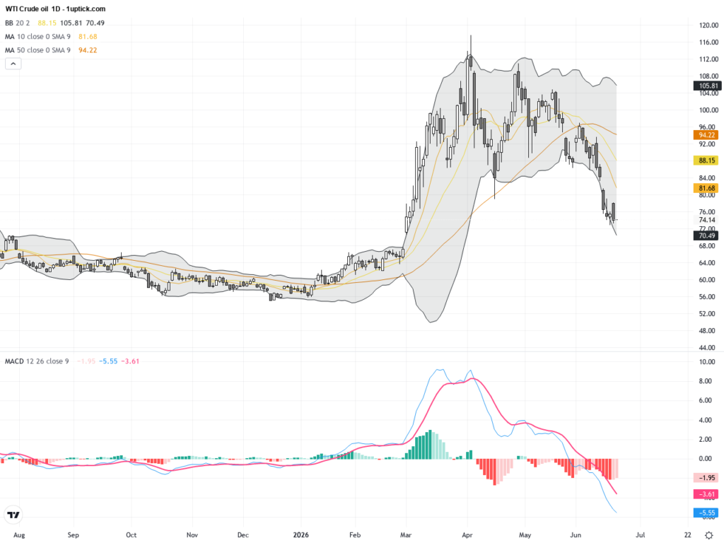
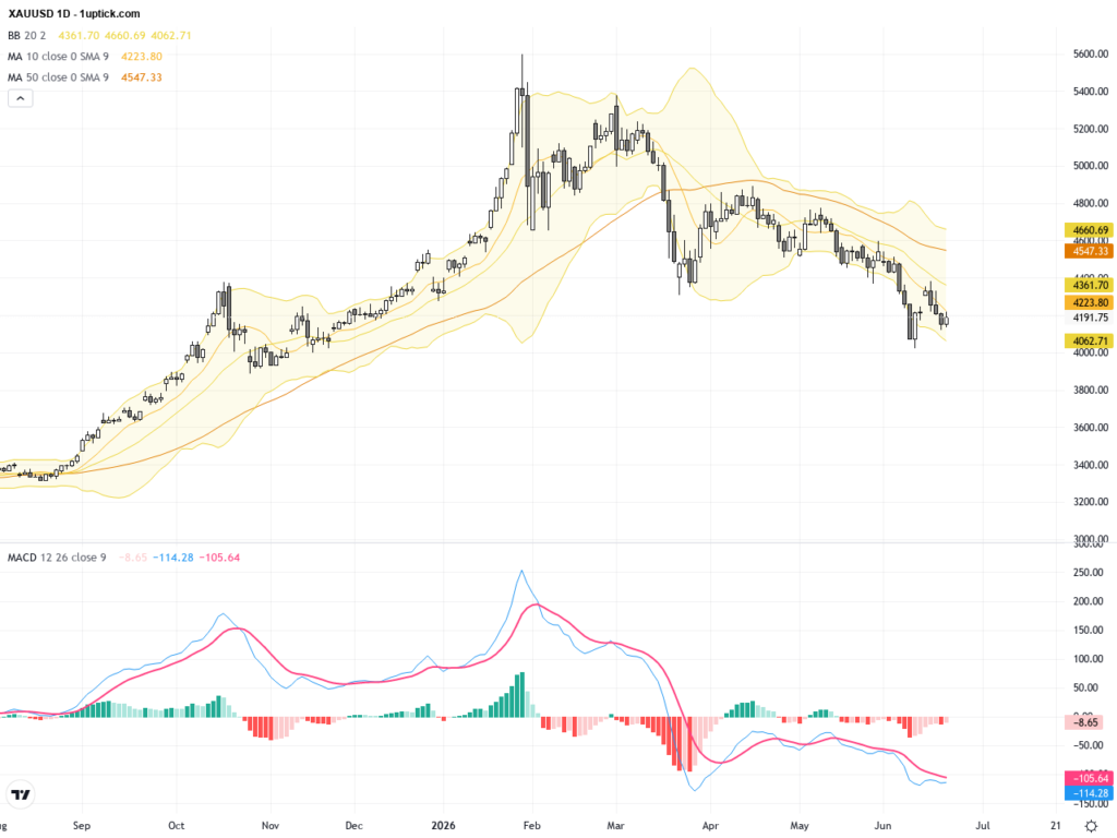
step_num: 2, heading: Build Regime-Conditional Return and Risk Profiles, content: Analyze historical performance of your target instruments across different regimes. For example, commodity currencies (AUD, CAD, NOK) typically outperform in Reflation regimes while underperforming in Deflation. Gold tends to excel during Stagflation and uncertainty. Create a matrix showing expected returns, volatilities, and correlations for each asset class under each regime.

step_num: 3, heading: Develop Regime Detection Algorithms, content: Implement quantitative regime detection using methods such as Hidden Markov Models, threshold-based rules on macro indicators, or machine learning classifiers trained on historical regime data. Your algorithm should output regime probabilities rather than binary classifications, allowing for gradual portfolio adjustments. Backtest regime detection accuracy across multiple market cycles.

step_num: 4, heading: Create Regime-Adaptive Risk Limits, content: Adjust your risk parameters based on detected regimes. During high-uncertainty or transition periods, reduce gross exposure by 20-40% and tighten stop-losses. In favorable regimes with clear trends, you may expand risk budgets. Define specific VaR limits, position size caps, and correlation assumptions for each regime in your risk policy document.

step_num: 5, heading: Implement Smooth Regime Transition Mechanisms, content: Avoid abrupt portfolio changes when regimes shift. Use probability-weighted blending where portfolio weights reflect the probability distribution across regimes. Implement transaction cost-aware rebalancing that only triggers when regime probabilities cross significant thresholds (e.g., 70%). This prevents whipsawing during ambiguous periods.

Part 3: Building a Risk Budgeting Framework for Multi-Asset Trading

step_num: 1, heading: Establish Your Total Risk Budget, content: Define the maximum portfolio volatility or Value-at-Risk you are willing to accept, typically expressed as annual volatility (e.g., 10-15% for moderate risk) or daily VaR at 95% confidence. This top-down risk budget should align with your investment objectives, time horizon, and stakeholder constraints. Document the rationale and approval process for any changes to this budget.

step_num: 2, heading: Decompose Risk Budget Across Asset Classes, content: Allocate your total risk budget across FX, commodities, and any other asset classes in your portfolio. Consider strategic allocation based on expected risk-adjusted returns and diversification benefits. A typical allocation might be 40% to FX majors, 25% to commodity currencies, 20% to precious metals, and 15% to energy commodities. This allocation should be reviewed quarterly.

step_num: 3, heading: Implement Risk Parity Principles, content: Within each asset class, size positions so that each contributes equally to portfolio risk, not equal dollar amounts. Calculate the marginal contribution to risk (MCTR) for each position using the formula: MCTR = weight × (covariance with portfolio / portfolio volatility). Rebalance when individual position risk contributions deviate significantly from targets.

step_num: 4, heading: Build Risk Budget Monitoring Infrastructure, content: Deploy real-time risk monitoring that tracks actual risk consumption against budgets at portfolio, asset class, and individual position levels. Create utilization dashboards showing percentage of risk budget used. Implement automatic alerts when utilization exceeds 80% or when projected utilization based on current market conditions approaches limits.

step_num: 5, heading: Establish Risk Budget Governance Procedures, content: Define clear escalation procedures when risk budgets are breached. Specify who has authority to approve temporary budget increases and under what circumstances. Create a risk committee that reviews budget allocations monthly and has authority to reallocate across strategies. Document all exceptions and their outcomes for continuous improvement.

Part 4: Using Dynamic Correlations for Position Sizing in Forex and Commodities

step_num: 1, heading: Select Appropriate Dynamic Correlation Models, content: Choose models that capture time-varying correlations effectively. DCC-GARCH models are industry standard, balancing accuracy with computational efficiency. For higher frequency trading, consider EWMA (Exponentially Weighted Moving Average) correlations with decay factors between 0.94-0.97. For longer horizons, regime-switching correlation models may be more appropriate.

step_num: 2, heading: Calibrate Model Parameters, content: Estimate model parameters using historical data spanning multiple market cycles. For DCC-GARCH, use maximum likelihood estimation on at least 5 years of daily data. Validate parameters through out-of-sample testing across different market conditions. Re-estimate parameters quarterly or when significant structural breaks occur in markets.

step_num: 3, heading: Integrate Dynamic Correlations into Position Sizing, content: Use the dynamically estimated correlation matrix in your portfolio optimization or risk budgeting calculations. When correlations between positions increase, automatically reduce position sizes to maintain target portfolio volatility. Implement the formula: Position Size = (Risk Budget × Target Correlation Contribution) / (Asset Volatility × Portfolio Correlation Factor).

step_num: 4, heading: Handle Correlation Estimation Uncertainty, content: Recognize that correlation estimates contain estimation error, especially during volatile periods. Apply shrinkage techniques that blend estimated correlations toward structured targets (such as constant correlation or factor-based structures). Use robust optimization techniques that account for estimation uncertainty in position sizing decisions.

step_num: 5, heading: Backtest and Validate Dynamic Sizing Approach, content: Compare portfolio performance using dynamic correlations versus static correlations across historical periods including stress events. Measure improvements in Sharpe ratio, maximum drawdown, and tail risk metrics. Ensure that transaction costs from more frequent rebalancing do not erode the benefits of dynamic sizing. Target rebalancing frequency that balances responsiveness with costs.

Part 5: Stress Testing a Diversified FX and Commodity Portfolio

step_num: 1, heading: Design Historical Stress Scenarios, content: Compile a library of historical stress events relevant to FX and commodities: 2008 Financial Crisis, 2011 Euro Crisis, 2014-15 Oil Crash, 2015 CNY Devaluation, 2020 COVID Crash, 2022 Russia-Ukraine Conflict. For each scenario, capture the price moves, volatility spikes, correlation changes, and liquidity conditions. Apply these historical moves to your current portfolio to measure potential losses.

step_num: 2, heading: Develop Hypothetical Stress Scenarios, content: Create forward-looking scenarios that may not have historical precedent: coordinated central bank intervention, major sovereign default, extreme climate event affecting commodity supply, or cyber attack on financial infrastructure. Work with economists and geopolitical analysts to develop plausible scenarios with specific market impact assumptions. Include both fast-moving crises and slow-burning structural shifts.

step_num: 3, heading: Implement Reverse Stress Testing, content: Instead of specifying scenarios and measuring losses, specify a loss threshold (e.g., 20% portfolio drawdown) and work backward to identify what market moves would cause such losses. This reveals hidden vulnerabilities and concentration risks that traditional stress tests might miss. Document the probability you assign to these scenarios materializing.

step_num: 4, heading: Model Liquidity Stress Conditions, content: Standard stress tests often assume positions can be liquidated at current prices. Incorporate liquidity stress by applying bid-ask spread widening, market impact costs for larger positions, and potential for trading halts in extreme scenarios. For less liquid commodity positions, model scenarios where exit takes multiple days with ongoing adverse price movement.

step_num: 5, heading: Integrate Stress Test Results into Risk Decisions, content: Use stress test results actively in portfolio management. Set limits so that stress losses remain within acceptable bounds (e.g., maximum 15% loss under any scenario). When stress exposures approach limits, proactively reduce positions or add hedges. Present stress test results to stakeholders monthly and update scenarios quarterly. Create action plans for each major stress scenario specifying exact steps to take if early warning indicators trigger.

Insider Insight: The most sophisticated risk management frameworks fail when they become too complex to execute under pressure. We have observed that institutions with simpler, well-rehearsed contingency plans consistently outperform those with elaborate models during actual stress events. Focus on building systems that degrade gracefully—when your correlation models fail, have fallback rules based on simple heuristics. When your regime detection is uncertain, default to more conservative positioning. The goal is not to predict every market move but to survive the scenarios you cannot predict. Additionally, the human element remains critical: ensure your trading team understands the rationale behind risk limits so they can make intelligent decisions when unprecedented situations arise. Finally, remember that diversification benefits are most valuable precisely when they are hardest to maintain—resist the urge to concentrate positions during calm markets when correlations appear stable.